
Features
Drainage Management Systems
Increasing drainage coefficients to respond to heavier rainfall
Comparing cost and benefit.
December 2, 2019 By Richard Cooke
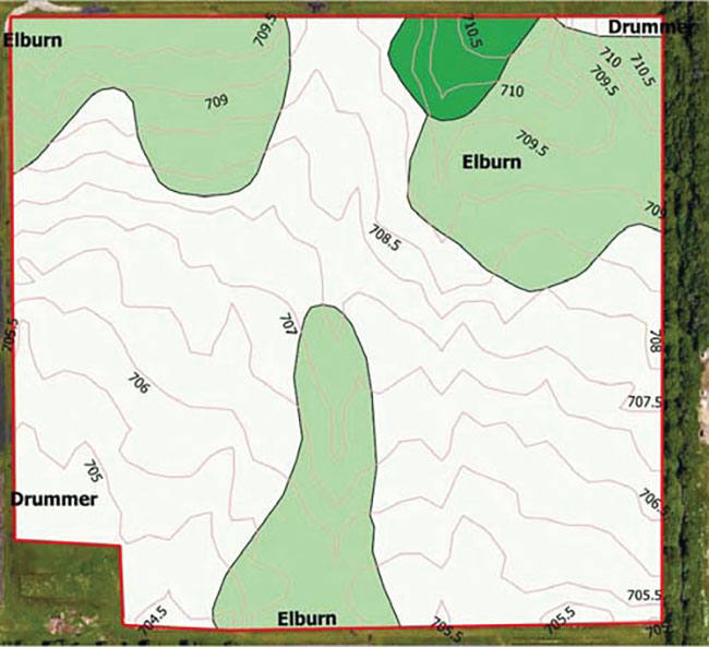 Figure 1. Field used for hydraulic analysis of three drainage system designs.
There were several large rainfall events this spring in Illinois, often on successive days, that left water ponded on even intensively drained fields for what seemed like forever.
Drainage systems in the state are typically designed using a 0.375 inch or a 0.5 inch drainage coefficient. The drainage coefficient is the depth of water removed from the soil in 24 hours, from a soil with an elliptic water table that initially touches the soil surface midway between the drains. This raises the question as to whether or not recommended design drainage coefficients should be increased. The answer lies in the realm of economics – optimizing cost and benefit. Such optimization requires an understanding of the hydraulic performance of various design options, among other things.
The drainage coefficient is the depth of water removed from the soil in 24 hours, from a soil with an elliptic water table that initially touches the soil surface midway between the drains.
A hydraulic analysis of the performance of three different drainage systems for the selected field are shown in Figure 1. This field is typical of many fields in Illinois – flat with a mixture of hydric soils that require drainage to be productive. In this instance the design is done for Drummer, the state soil and the most ubiquitous soil in the state. Because there is a ditch next to the field, the mains are short. Longer mains change the economic calculus, but the hydraulic analysis is very representative.
System A is a typical design for Drummer. The tiles are spaced 100 feet apart and put at an average depth of 3.5 feet. The resulting drainage coefficient is 0.375 inches. The tile spacing in System B (50 feet) is half that of System A, and the tiles are shallower (2.5 feet). This system represents a trend towards installing narrower, shallower systems with higher drainage coefficients, 0.91 inches in this instance.
In System C, the drainage coefficients are uncoupled, with 0.375 inches and 0.91 inches used for the laterals and mains, respectively. The analysis was performed for the first 24 hours after an event that saturates the soil and causes the water table to be flat at the soil surface. This scenario is likely after a rain event that exceeds the capacity of the main. The capacity of the main is not necessarily the same as the design drainage coefficient.

Figure 3. Layout and pipe sizes for drainage systems used for analysis.
The relationship between design drainage coefficient and main capacity is shown in Figure 3 (above). The main capacity corresponding to a 0.375 inches drainage capacity is 8.9 inches (Pipe a). However, since pipes sizes are standard, a 10 inches pipe would be used for this system. The main capacity for this 10 inches pipe is the drainage coefficient that makes the actual pipe size the same as the nominal pipe size (Pipe c). This value (0.512 inches) can be found by trial and error, or by using the goal seek function in the main sizing, Excel worksheet as demonstrated in Figure 3.
The capacity for the 15 inches main was 1.51 inches in this instance. A schematic of water table profiles from draining a flat water table is shown in Figure 4 (below). Firstly, the extent of the drawdown region, called the effective spacing, increases until it extends to midway between the drains. At this instant the effective spacing is the same as the actual drain spacing (red line in Figure 4). As time increases, the mid-plane water table height decreases. When the effective spacing is less than the actual drain spacing, the instantaneous drainage coefficient exceeds the design drainage coefficient.
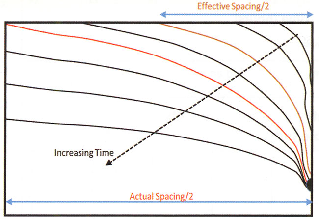
Figure 4. Water table profiles on one side of a lateral resulting from draining an initially flat-water table.
The maximum rate at which water leaves the profile is governed by the capacity of the main. At the instant the effective spacing equals the actual drain spacing, the instantaneous drainage coefficient is equal to the design drainage coefficient. As time progresses and the mid-plane water table height decreases, the instantaneous drainage coefficient is less than the design drainage coefficient.
The evolution for the effective spacing for Systems A and B are shown in Figure 5. For the deeper wider system, System A, it takes approximately nine hours for the effective spacing to equal the actual spacing. The corresponding time for the narrower, shallower system, System B, is approximately three hours.
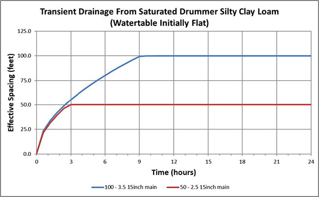
Figure 5. Effective spacing versus time from draining an initially flat-water table.
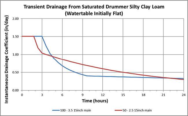
Figure 6. Instantaneous drainage coefficient versus time from draining an initially flat-water table.
The instantaneous drainage coefficients for the first 24 hours of drainage are shown in Figure 6. The capacity of the main controls the drainage for the first 3.0 hours and 1.8 hours, respectively, for Systems A and B. After these times the drainage rate is dictated by the transport properties of the soil.
The drainage rate in the deeper, wider system equals or exceeds that of the shallower, narrower system for the first 4.8 hours. After 24 hours, the drainage rate from the two systems are approximately equal, but drainage rate from the shallow system decreases faster than that for the deeper system.
The depth of water removed over the first 24 hours by each of the three systems is shown in Figure 7. The cumulative depths are 0.42 inches, 0.69 inches, and 0.58 inches, respectively, for Systems A, B, and C.
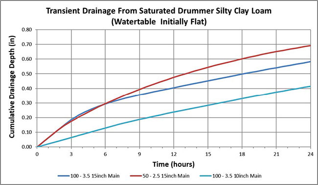
Figure 7. Instantaneous drainage coefficient versus time from draining an initially flat-water table.
System costs and 24-hour drainage rates are shown in Table 1. The unit pipe costs are representative industry standard. Unit pipe cost is often dependent on job size, decreasing as job size increases. The cost does not include the cost of making connections or of moving equipment. As mentioned earlier, these systems have short mains as they are next to a ditch. In reality, main costs can be significantly more, depending on the distance to be travelled to an outlet.
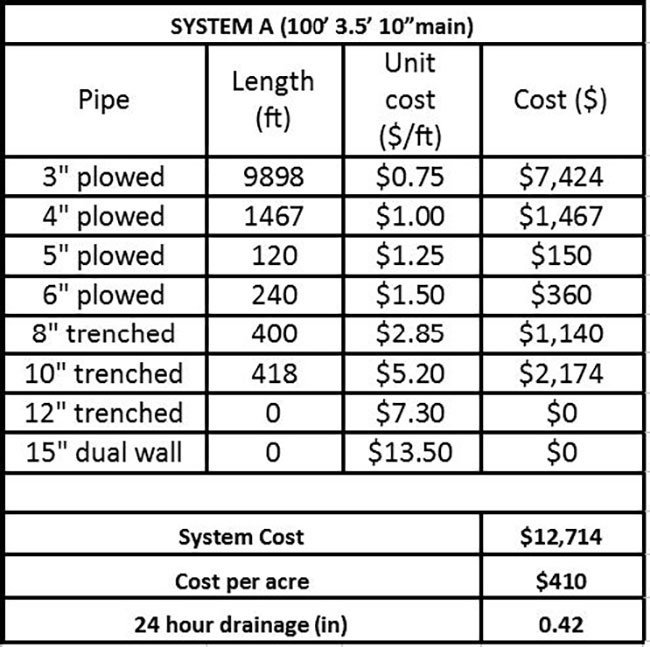
Table 1. Drainage Systems Costs.

Table 1. Drainage Systems Costs.
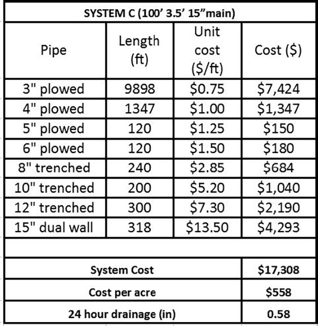
Table 1. Drainage Systems Costs.
The systems were designed using three inch laterals were possible. With the laterals being steep and much shorter than the lengths that would cause them to flow at capacity, it is unlikely that the laterals will restrict flow, even at high instantaneous drainage rates. However, four inch laterals are much less likely to restrict flow than three inch laterals, so that might be a design consideration. The most cost effective of the three systems seem to be System C, in which the drainage coefficients for mains and laterals were uncoupled. This should be a consideration in designing drainage systems for faster drainage after large events. Another option would be to increase the depth of narrower systems. In this instance, for example, if the narrow system were placed 3.5 feet deep, the drainage coefficient would be 1.34 inches, which is less than the 1.51 inches limit for a 15-inch main. The cost, therefore, would not change much. However, the 24-hour drainage would increase to 1.0 inches, a 45 percent increase over the 24-hour drainage of the shallower system with the same spacing.
In many cases system depth is limited by the depth of the outlet. In instances where this is not so, it seems that designing the system with a drainage coefficient that equalizes the actual and nominal pipe sizes would be the most cost effective. Cost effectiveness could also be increased by uncoupling the drainage coefficients for mains and laterals.
Richard Cooke is an associate professor of agricultural and biological engineering at the University of Illinois.
One of his focus areas includes optimizing subsurface drainage system design, where he works to increase the efficiency of drainage-related best management practices and develops protocols for their design. He also develops techniques to simplify the extraction of elevation data from a pulsed laser system (LiDAR) images, and creates rainfall harvesting systems to extend cropping into the dry season in Sierra Leone.
He has proposed developing two routines for the design of subsurface drainage systems, which will maximize soil storage volume without adversely affecting crop yields.
Print this page